Testing positional accuracy underwater, revisited

I had the opportunity to test positional accuracy while underwater.  Amazingly, I did not even have to get wet!  While I was doing some GIS work with the excellent faculty at the University of Hamburg, I walked through the St. Pauli Elbe Tunnel while collecting a track.  As I did so, I reflected on the fascinating cultural and physical geography of this 1911 engineering masterpiece that is still in use:  The tunnel is 426 m (1,398 ft) long; it was a technical sensation when constructed; photos at the entrance show Kaiser Wilhelm II dedicating it.  It connected central Hamburg on the north side of the river with the docks and shipyards on the south side of the River Elbe.  The most amazing part was the four massive elevators, capable of carrying bikes and whole vehicles, and of course, 100 years ago, carriages and horses.  These elevators and tunnel are still functional and being used today!  For more information on this experiment, see my new video on the Our Earth channel here.

While pondering these thoughts, I collected a track in the Runkeeper app, and mapped it as a GPX file in ArcGIS Online as a 2D webmap and as a shapefile in a 3D scene.  I wanted to test how spatially accurate a track underwater would be, in the x and y dimensions, but also in the z dimension.  First, let’s consider the x and y:  As I walked through the tunnel 24 m (80 ft) beneath the surface through one of the two 6 m (20 ft) diameter tubes, I expected the my app to lose sight of the GPS, Wi-Fi, and cell phone towers, but I did not know how far off my position would be.   My recent experiments on an above-ground track gave me a ray of hope that perhaps my position would be recorded as somewhere in Germany rather than in the North Sea or the Atlantic Ocean.

I was told by a local source who said that the tunnels are 8 m below the bottom of the river, and the depth of the river is 8 m here as well (this depth here allowed Hamburg to become of the largest container ports in the world).  Thus, above me was about 4 meters of airspace, 8 meters of sediment (glacial, in this area), and 8 meters of water for a total of 20 meters above me.  The elevation at the water surface here is approximately 5 m above sea level.  Thus, my elevation in the tunnel should be 5 – 20 = -15 meters.

My results as a 2D webmap and as a 3D scene are shown below.  As is evident, the recorded elevations are all above sea level, at around 4 meters, so they were 15+4=19 meters off of my actual elevation in the tunnel.

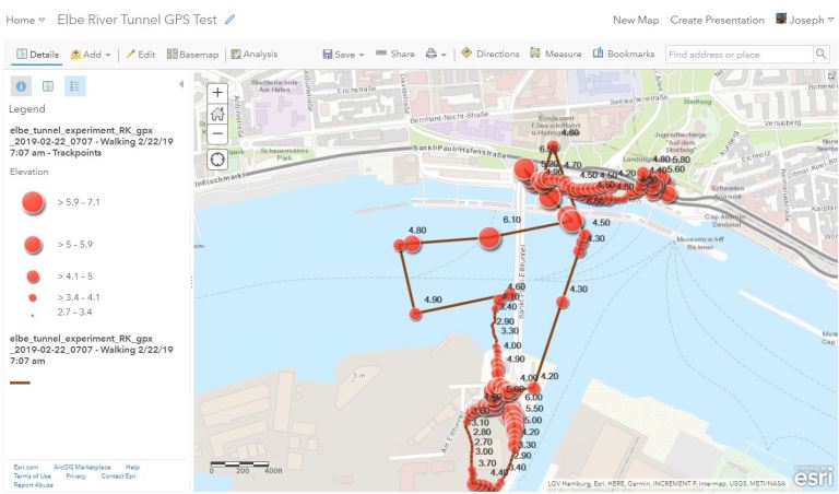A 2D map in ArcGIS Online showing the results of my experiment, with elevations in meters above sea level shown as labels. 

Feel free to open and interact with the data!  For example, to test the X and Y:  Using the measure tool, measure the distance between the tunnel as shown on the OpenStreetMap basemap and the position recorded by my track.  As I left the train station on the north side, my position was fairly accurately recorded, but once I descended the stairs into the tunnel, my position was off to the east by about 140 meters, and then shifted to the west and was off by about 240 meters.  But as I continued walking south, for the last 1/3 of my trek through the tunnel, my XY positional accuracy was only off by 50 meters.   I ascended the stairs and circled the parking lot on the south side, and was only 1 to 2 meters off once more.  I descended into the tunnel and walked north.  This time, my position was about 100 meters off, becoming worse as I kept walking.  My position overcorrected 80 meters to the north as I ascended the stairs, and “settled back” to being a few meters off as I walked to the train station.

To test the Z position:  The elevations were, as I suspected, not displaying their correct number below sea level; that is, 15 meters below sea level. However, you can see that the elevations are actually quite close to the elevation of the surface of the river in this area; at about 4.5 meters.

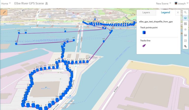A 3D scene in ArcGIS Online showing the results of my experiment, with elevations in meters above sea level shown as labels and symbolized as cylinders.   Feel free to open and interact with this 3D scene!

Overall, with only a smartphone and a fitness app, displaying the data in ArcGIS Online, I was rather pleased with the fact that my positions all around were usually only in the tens or a few dozen meters off of true. This aligns with my recent reports of above-ground experiments and is further evidence of the improvements in spatial accuracy with all location based services.

Interested in further exploration?  See the evidence of my field trip in the photographs below.

The Elbe River as it appears near the tunnel.

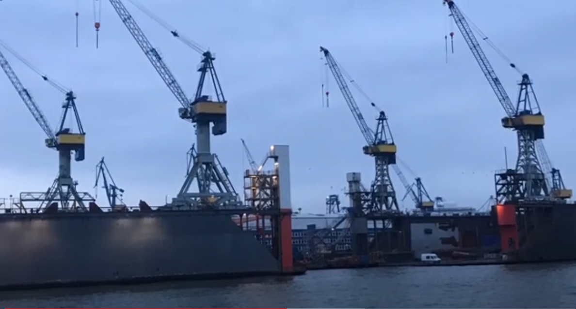
Part of the enormous container port on the south bank of the Elbe.

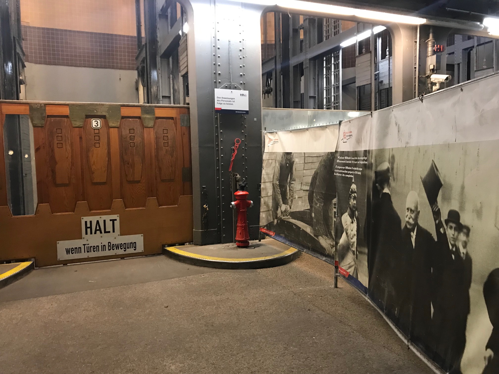
The very large elevators that carry pedestrians, bicycles, and even vehicles from the street level to the level of the tunnels.  This one is at the north side of the river with a photo of the opening ceremony with Kaiser Wilhelm II dedicating it.

Standing at the entrance to the tunnel; this photo also shows a few of the glazed terra cotta art sculptures on the left, and in the distance on the right.

Now, go conduct your own accuracy experiments!

–Joseph Kerski

Be a Wise Consumer of Fun Posts, too!

Around this time of year, versions of the following story seem to make their way around the internet:

The passenger steamer SS Warrimoo was quietly knifing its way through the waters of the mid-Pacific on its way from Vancouver to Australia. The navigator had just finished working out a star fix & brought the master, Captain John Phillips, the result. The Warrimoo’s position was LAT 0º 31′ N and LON 179 30′  W.  The date was 31 December 1899.

“Know what this means?” First Mate Payton broke in, “We’re only a few miles from the intersection of the Equator and the International Date Line”.  Captain Phillips was prankish enough to take full advantage of the opportunity for achieving the navigational freak of a lifetime.  He called his navigators to the bridge to check & double check the ships position.  He changed course slightly so as to bear directly on his mark.  Then he adjusted the engine speed. The calm weather & clear night worked in his favor. 

At midnight the SS Warrimoo lay on the Equator at exactly the point where it crossed the International Date Line! The consequences of this bizarre position were many:  The forward part (bow) of the ship was in the Southern Hemisphere & the middle of summer. The rear (stern) was in the Northern Hemisphere & in the middle of winter.  The date in the aft part of the ship was 31 December 1899.  Forward it was 1 January 1900.  This ship was therefore not only in two different days, two different months, two different years, two different seasons, but in two different centuries – all at the same time.

I have successfully used many types of geographic puzzles with students and with the general public over the years, and I enjoy this story a great deal.  But in keeping with our reminders on this blog and in our book to “be critical of the data,” reflections on the incorrect or absent aspects to this story can be instructive as well as heighten interest. The SS Warrimoo was indeed an actual ship that was built by Swan & Hunter Ltd in Newcastle Upon Tyne, UK, in 1892, and was sunk after a collision with a French destroyer during World War I in 1918.  Whether it was sailing in the Pacific in 1899, I do not know.

The version of this story on CruisersForum states that it is “mostly true.”  What lends itself to scrutiny?  Let us investigate a few of the geographic aspects in the story.

First, the statement, “working out a star fix” leaves out the fact that chronometers were used to work out the longitude, rather than a sextant.  (And I highly recommend reading the book Longitude by Dava Sobel).  Second, the International Date Line (IDL) as we know it today was not in place back in 1899.  The nautical date line, not the same as the IDL, is a de jure construction determined by international agreement. It is the result of the 1917 Anglo-French Conference on Time-keeping at Sea, which recommended that all ships, both military and civilian, adopt hourly standard time zones on the high seas. The United States adopted its recommendation for U.S. military and merchant marine ships in 1920 (Wikipedia).

Third, the distance from LAT 0º 31′ N and LON 179 30′ W to LAT 0º 0′ N and LON 180′ W is about 42 nautical miles, and the ship could have traveled at a speed of no more than 20 knots (23 mph).  Therefore, conceivably, the ship could have reached the 0/180 point in a few hours, but whether it could have maneuvered in such a way to get the bow and stern in different hemispheres is unlikely, given the accuracy of measurement devices at the time.  Sextants have an error of as at least 2 kilometers in latitude, and chronographs about 30 kilometers in longitude. Or, they could already have reached the desired point earlier in the day and not have known it.  Even 120 years later, in my own work with GPS receivers at intersections of full degrees of latitude and longitude, it is difficult to get “exactly” on the desired point:  Look carefully at the GPS receiver in my video at 35 North Latitude 81 West Longitude as an example.  An interesting geographic fact is that, going straight East or West on the Equator along a straight line, it is possible to cross the dateline three times (see map below).

Our modern digital world is full of fragments that are interesting if not completely accurate, but as GIS professionals and educators, I think it is worth applying “be critical of the data” principles even to this type of information.  The story is still interesting as a hypothetical “what could have happened” and provides great teachable moments even if the actual event never occurred.

The International Date Line (CC BY-SA 3.0, https://commons.wikimedia.org/w/index.php?curid=147175).

Testing positional accuracy underwater

I recently had the opportunity to test positional accuracy while underwater.  And I did not even have to get wet!  While I was doing some GIS work with the excellent faculty at the University of Hamburg, I walked through the St. Pauli Elbe Tunnel while collecting a track.  As I did so, I reflected on the fascinating cultural and physical geography of this 1911 engineering masterpiece that is still in use:  The tunnel is 426 m (1,398 ft) long; it was a technical sensation when constructed; photos at the entrance show Kaiser Wilhelm II dedicating it.  It connected central Hamburg on the north side of the river with the docks and shipyards on the south side of the river Elbe.  The most amazing part was the four massive elevators, capable of carrying bikes and whole vehicles, and of course, 100 years ago, carriages and horses.  These elevators and tunnel are still functional and being used today!

While pondering these thoughts, I collected a track in the Runkeeper app, and mapped it as a GPX file in ArcGIS Online as a 2D webmap and as a shapefile in a 3D scene.  I wanted to test how spatially accurate a track underwater would be, in the x and y dimensions, but also in the z dimension.  First, let’s consider the x and y:  As I walked through the tunnel 24 m (80 ft) beneath the surface through one of the two 6 m (20 ft) diameter tubes, I expected the my app to lose sight of the GPS, Wi-Fi, and cell phone towers, but I did not know how far off my position would be.   My recent experiments on an above-ground track gave me a ray of hope that perhaps my position would be recorded as somewhere in Germany rather than in the North Sea or the Atlantic Ocean.

I was told by a local source who said that the tunnels are 8 m below the bottom of the river, making the water 16 m deep here (this depth here allowed Hamburg to become of the largest container ports in the world).  Thus, above me was 8 m of sediment (glacial, in this area), and 16 m of water for a total of 24 meters above me.  The elevation at the water surface here is approximately 5 m above sea level.  Thus, my elevation in the tunnel should be 5 – 24 = -19 meters, minus 3 more meters because I was standing on the bottom of the tunnel rather than the top, so -22 meters.

My results as a 2D webmap and as a 3D scene are shown below.  As is evident, the recorded elevations are all above sea level, at around 4 or 5 meters, so they were 22+5=27 meters off of my tunnel elevation.

A 2D map in ArcGIS Online showing the results of my experiment, with elevations in meters above sea level shown as labels. 

Feel free to open and interact with the data!  For example, to test the X and Y:  Using the measure tool, measure the distance between the tunnel as shown on the OpenStreetMap basemap and the position recorded by my track.  As I left the train station on the north side, my position was fairly accurately recorded, but once I descended the stairs into the tunnel, my position was off to the east by about 140 meters, and then shifted to the west and was off by about 240 meters.  But as I continued walking south, for the last 1/3 of my trek through the tunnel, my XY positional accuracy was only off by 50 meters.   I ascended the stairs and circled the parking lot on the south side, and was only 1 to 2 meters off once more.  I descended into the tunnel and walked north.  This time, my position was about 100 meters off, becoming worse as I kept walking.  My position overcorrected 80 meters to the north as I ascended the stairs, and “settled back” to being a few meters off as I walked to the train station.

To test the Z position:  The elevations were, as I suspected, not displaying their correct number below sea level; that is, 19 meters below sea level. However, you can see that the elevations are actually quite close to the elevation of the surface of the river in this area; at about 4.5 meters.

A 3D scene in ArcGIS Online showing the results of my experiment, with elevations in meters above sea level shown as labels and symbolized as cylinders.   Feel free to open and interact with this 3D scene!

Overall, with only a smartphone and a fitness app, displaying the data in ArcGIS Online, I was rather pleased with the fact that my positions all around were usually only in the tens or a few dozen meters off of true. This aligns with my recent reports of above-ground experiments and is further evidence of the improvements in spatial accuracy with all location based services.

Interested in further exploration?  See the evidence of my field trip in the photographs below.

The enormous elevators that carry pedestrians, bicycles, and even vehicles from the street level to the level of the tunnels.  This one is at the north side of the river with a photo of the opening ceremony with Kaiser Wilhelm II dedicating it.

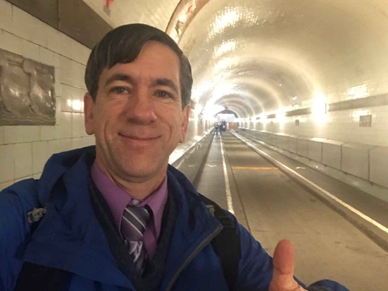Standing at the entrance to the tunnel; photo also shows one of the glazed terra cotta art sculptures.

Now, go conduct your own accuracy experiments!

–Joseph Kerski

 

Track on Track, Revisited: Spatial Accuracy of Field Data

Back in 2014, I tested the accuracy of smartphone positional accuracy in a small tight area by walking around a track.  During a recent visit to teach GIS workshops at Carnegie Mellon University, I decided to re-test, again on a running track.  My hypothesis was that triangulation off of wi-fi hotspots, cell phone towers, and the improved GPS constellation would have improved the spatial accuracy of my resulting track over those intervening years.

After an hour of walking, and collecting the track on my smartphone with a fitness app (Runkeeper), I uploaded my track as a GPX file and created a web map showing it in ArcGIS Online.  Open this map > use bookmarks > navigate to the Atlanta and Pittsburgh (Carnegie Mellon University) locations (also shown on the graphic below on the left and right, respectively).   Once I mapped my data, my hypothesis was confirmed:  I kept to the same lane on the running track, and the width of the resulting lines averaged about 5 meters, as opposed to 15 meters on the track from four years ago.  True, the 2014 track variability was no doubt in part because I was surrounded by tall buildings on three sides (as you can see in my video that I recorded at the same time) , while the building heights on the Carnegie Mellon campus were much lower.  However, you can measure for yourself on the ArcGIS Online map linked above and see the improvement over those two tracks taken just 4 years apart.

I did another test while at Carnegie Mellon University–during my last lap on the track, I moved to the inside lane.   This was 5 meters inside the next-to-outer lane where I completed my other laps.  I wanted to see whether this shift would be visible on the resulting map.  It is!  The lane is clearly visible on the map and on the right side of the graphic below, which I labeled as “inside lane.”

To explore further, on the map above, go to > Contents, to the left of the map, and turn on the World Imagery Clarity layer.   Then use the Measure tool to determine how close the track is to the satellite imagery (which isn’t perfect either, but see teachable moments link below).  You will find that at times the track was 0.5 meters from the image underneath Lane 1, and at other times 3.5 meters away.

Both tracks featured “zingers” – lines stretching away from the actual walking tracks, resulting from points dropped as I exited the nearby buildings and walked outside, as my location based service first got its bearing.  But again, an improvement was seen:  The initial point was 114 meters off in 2014, but in 2018, only 21.5 meters.  In both cases, as I remained outside, the points became more accurate.  When you collect data, the more time you spend on the point you are collecting, typically the more spatially accurate that point is.

Comparison of tracks taken with the same application (RunKeeper) on a smartphone four years apart illustrate the improvements in positional accuracy over that time. 

To dig deeper into issues of GPS track accuracy and precision, see my related essay on errors and teachable moments in collecting data, and on comparing the accuracy of GPS receivers and smartphones and mapping field collected data in ArcGIS Online here.

Location based services on the smartphone still do not yet deliver the spatial accuracy for laying fiber optic cable or determining differences in closely-spaced headstones in cemeteries (unless a device such as Bad Elf or a survey-grade GPS is used).  Articles are appearing that predict spatial accuracy improvements in smartphones.  Even today, though, I was quite pleased with my track’s spatial accuracy, particularly in 2018.  I was even more pleased considering that I had the phone in my pocket most of the time I was walking.  I did this in part because it was cold, and cold temperatures tend to rapidly deplete my cell phone’s battery (which is unfortunate, and the subject of other posts, many of which sport numerous adds, so they are not listed here).   Happy field data collection and mapping!

–Joseph Kerski